I see a different measurement reported by the THD block than what I measure with the same frequency in a Scope on the same current meter. I’ve attached a screenshot (0.008 from THD block and 0.014 on the scope). Am I missing something? Shouldn’t these match?
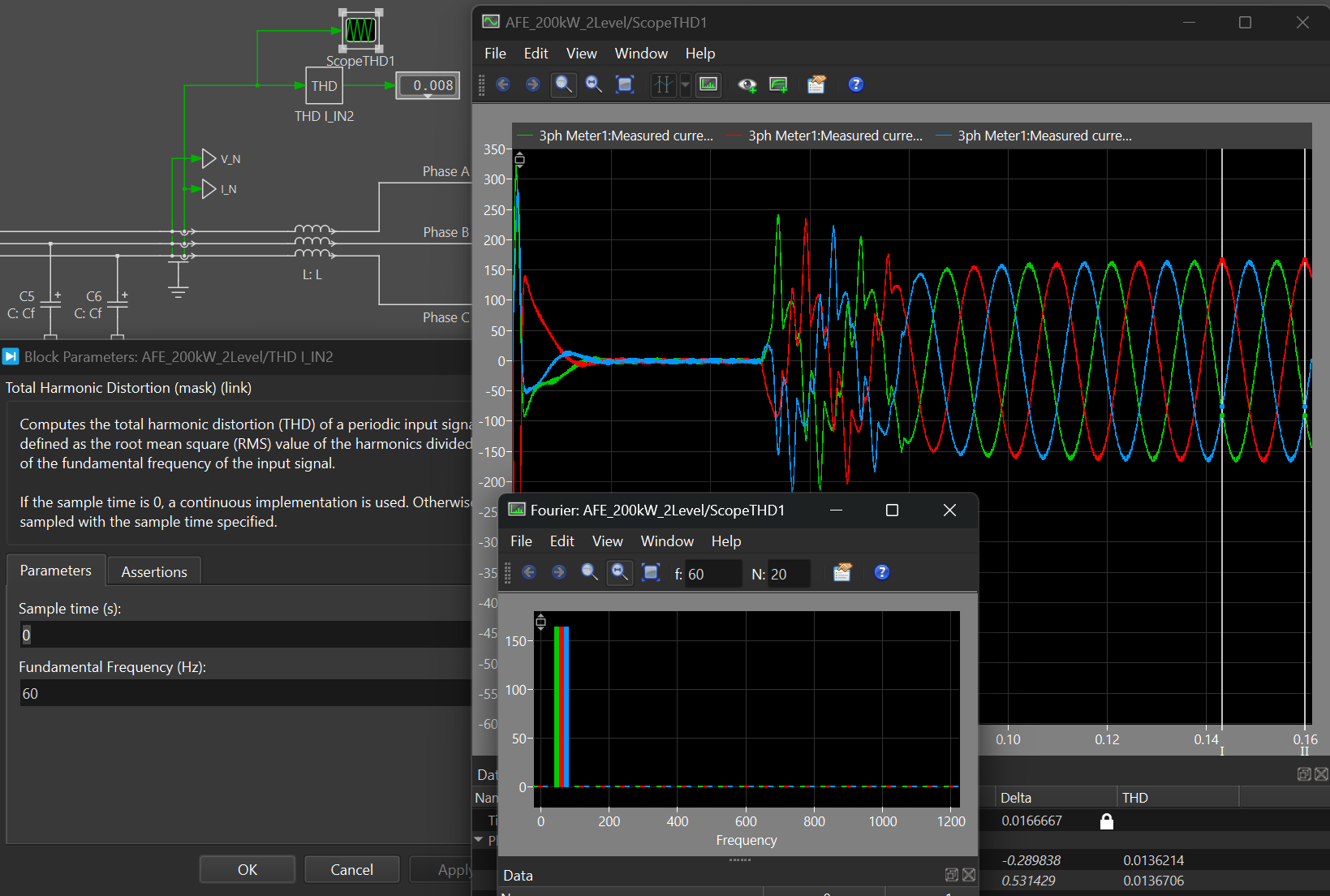
Yes, generally speaking they should match. One key difference is the PLECS Scope analyzes the simulation results shown in the scope while the THD block performs operations as the model runs, so this discrepancy likely comes down to the solver settings.
Could you please share a model to recreate this? You are welcome to send a direct message or email to me (simply my last name @plexim.com).
Hi Bryan,
Sending you an email now with a model.
Thanks,
Ben
Ben and I were able to analyze his model. The analysis confirms that the numerical behavior of the solver is the reason the THD results. For numerical issues, it often comes down to the peculiarities / characteristics of the model.
According to the THD block’s documentation, the THD is calculated as:
THD=\sqrt{\frac{\sum_{v\ge2}^\infty U_v^2 }{U_1^2}}=\sqrt{\frac{U_{rms}^2-U_0^2-U_1^2}{U_1^2}}
Where U_v is the v \mathrm{th} harmonic and U_{rms} is the overall RMS value.
In Ben’s model the U_{rms}^2 and U_1^2 values are quite close. A <0.01% error in these signals results in a 50% change in the THD value.
We can change the Relative Tolerance settings to force the solver to be more accurate. This increases the run-time, but we can set the relative tolerance quite low (e.g 1e-7 or lower) to get a known-good result. We can also change the solver type to see how it impacts accuracy and speed.
Below is the output from a simulation script that compares solver type, relative tolerance, THD from the block, THD from the PLECS Scope, and the approximate execution time of the model. The THD at two different points in Ben’s model are compared.
Solver	RelTol	ThdBlock1	ThdScope1	ThdBlock2	ThdScope2	Exec.Time
radau	 0.001 	0.012785	0.015776	0.007900	0.013708	 4.8
radau	 1e-07 	0.015759	0.015873	0.013578	0.013708	17.0
radau	 1e-08 	0.015876	0.015877	0.013703	0.013708	24.8
dopri	 0.001 	0.000000	0.015960	0.013708	0.013708	 2.6
dopri	 1e-05 	0.015752	0.015856	0.013708	0.013708	 4.4
dopri	 1e-07 	0.015879	0.015875	0.013708	0.013708	 8.8
One can conclude that a non-stiff (DOPRI) solver with an 1e-5 relative tolerance is both accurate and runs fast. Furthermore, the Scope results are less dependent on the solver settings and don’t slow down the run-time of the model as it is a post processing step, so you may just want to rely on that measurement.
Hopefully this provides a workflow where you and future users can feel more confident in the reported THD.
The simple simulation script for PLECS Standalone is below:
function runTestCase(Solver,RelTol)
    % Run simulation with different solver settings.
    % Get THD block results at last time step.
    % Get THD scope results over last period.
	TimeSpan = 0.25;
    opts=struct('SolverOpts',struct('Solver',Solver,'RelTol',RelTol,'OutputTimes',TimeSpan,'TimeSpan',TimeSpan));
	tic
	r=plecs('simulate',opts);
	executionTime = toc;
	thdBlock = r.Values;
	scopeData = plecs('scope', './ScopeTHD', 'GetCursorData', [(TimeSpan-1/60) TimeSpan],'thd');
	thdScope = [scopeData.cursorData{1}{1}.thd;scopeData.cursorData{2}{1}.thd];
	printf('%s\t %.1g \t%3.6f\t%3.6f\t%3.6f\t%3.6f\t%4.1f\n',Solver,RelTol,thdBlock(1),thdScope(1),thdBlock(2),thdScope(2),executionTime)
end

printf('Solver\tRelTol\tThdBlock1\tThdScope1\tThdBlock2\tThdScope2\tExec.Time\n')
runTestCase('radau',1e-3);
runTestCase('radau',1e-7);
runTestCase('radau',1e-8);
runTestCase('dopri',1e-3);
runTestCase('dopri',1e-5);
runTestCase('dopri',1e-7);