DQ Transformation
Multiple conventions exist for the DQ (direct-quadrature) transformation, differing in frame alignment and axis ordering. The choice of convention affects the resulting equations and signs in the model.
The convention used in PLECS is shown in Fig. 1 highlighting:
- The rotor’s electrical angle \theta_e is measured from the phase A flux to the rotor’s angular position.
- The D-axis is aligned with the stator’s phase A winding flux linkage when the rotor’s electrical angle \theta_e=0.
- The Q-axis leads the D-axis by 90 degrees.
- Positive Q-axis current (i_q>0) produces positive electrical torque.
- The D-axis corresponds to the magnetic north of the rotor, whether that is generated by permanent magnets or a positive field winding current.
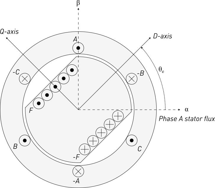
Figure 1: Electric Machine Axis Conventions
This behavior corresponds to the formulation of the abc to stationary (\alpha\beta) and abc to rotating (DQ) transforms in the PLECS manual:
If you implement a controller designed for a different convention, you may need to swap i_d and i_q references, negate certain terms, or adjust the angle transformation by \pm 90^\circ.
Electrical and Mechanical Quantities
The electric rotor angle \theta_e is used in the DQ transformation and appears throughout the machine equations. However, one can only directly measure the machine shaft’s mechanical quantities using the Rotational Speed Sensor and Angle Sensor (or measure these quantities using the PLECS Probe).
The mechanical quantities for speed \omega_m in rad/s and angle \theta_m in rads often need to be converted to the corresponding electrical quantities by multiplying by the number of pole-pairs p:
Common mistakes include:
- Using mechanical angle and speed when electrical quantities are required.
- Use of alternative units such as degrees for angle or RPM for speed without converting to correct SI units of angular frequency in rad/s and angular position in rads.
Generator and Motor Operation
All machines in PLECS can operate in either motor or generator mode. If the mechanical torque has the same sign as the rotational speed the machine is operating in motor mode, otherwise in generator mode.
The table below summarizes the different motor and generator operating modes, using the convention that a positive torque and speed is the forward mode.
| Quadrant | Speed | Torque | Mode | Power Flow |
|---|---|---|---|---|
| I | + | + | Forward motoring | Electrical → Mechanical |
| II | + | − | Forward generating (braking) | Mechanical → Electrical |
| III | − | − | Reverse motoring | Electrical → Mechanical |
| IV | − | + | Reverse generating (braking) | Mechanical → Electrical |
Current Direction Convention
Current direction conventions determine the sign of electrical power and must be consistent throughout the model. The PLECS convention is:
- Positive current flows into the machine’s stator terminals from the external electrical network
- This matches the standard motor convention used in most electrical machinery textbooks
- Positive real power (P > 0) flows into the machine in motor mode
Understanding Back EMF Constant, Torque Constant, and Flux Linkage
The Permanent Magnet Synchronous Machine (PMSM) and Brushless DC Machine (BLDC) components in the PLECS library require users to enter a parameter characterizing the strength of magnetic flux.
Motor manufacturers use various conventions for specifying back EMF constant K_e, torque constant K_t, and permanent magnet flux \phi. The most common variations involve:
- Voltage measurement: Line-to-neutral vs. line-to-line
- Voltage amplitude: Peak vs. RMS quantities
- Speed units: Mechanical rad/s vs. mechanical RPM vs. mechanical kRPM
- Torque units: SI units such as newton meters (N-m) vs. imperial units such as ounce-inches (oz.-in) or pound-feet (lb-ft)
PLECS Conventions
In PLECS the BLDC (Simple) machine’s back EMF constant K_e is defined in units of V_{LN,pk} /\omega_m where \omega_m is in mechanical rad/s. The BLDC model uses K_e because it’s more directly related to measurable back EMF, especially when considering both trapezoidal and sinusoidal back EMF shapes.
The PMSM machines in PLECS use the flux induced by the permanent magnet \phi in units of volt-seconds (Vs) or webers (Wb). The induced flux is a logical choice as it appears in the DQ frame flux linage equations.
Note that these parameters all represent the same basic physical phenomena - the magnetic coupling of the rotor magnets and the stator.
For machines with sinusoidal back EMF the relationship between the flux linkage and back EMF constant is: K_e = p\phi where p is the number of pole-pairs.
Conversion Table for Common K_e Datasheet Formats
The table below provides the coefficients to convert between common datasheet formats for K_e and PLECS back EMF convention for the BLDC (Simple) machine model with Sinusoidal flux. The equivalent PMSM flux linkage coefficient requires accounting for the number of pole-pairs with an additional 1/p scaling factor.
| Datasheet Format | Conversion to PLECS Ke | Notes |
|---|---|---|
| Vln,peak / (rad/s) | 1 | Direct match - no conversion needed |
| Vll,peak / (rad/s) | 1/{\sqrt{3}} | Convert line-to-line to line-to-neutral |
| Vln,RMS / (rad/s) | \sqrt{2} | Peak is \sqrt{2} RMS for sinusoidal waveforms |
| Vll,RMS / (rad/s) | \sqrt{2/3} | Combine both conversions |
| Vln,peak / RPM | \frac{60}{2\pi} | Convert RPM to rad/s |
| Vll,peak / kRPM | \frac{60}{2\pi}\frac{1}{1000}\frac{1}{\sqrt{3}} | Most common industrial format |
| Vll,RMS / kRPM | \frac{60}{2\pi}\frac{1}{1000}\sqrt{\frac{2}{3}} | Combines RMS, line-to-line, and kRPM |
The attached model shows the conversion from Vll,peak/kRPM to equivalent parameters for the PMSM and BLDC machine models, and compares the open winding line-to-line voltages at 1 kRPM to the specified constant. Note that the peak line-to-neutral voltage induced by the back EMF is K_e\omega_m.
Ke_conversion_example.plecs (14.4 KB)
Torque Constant
Some datasheets provide a torque constant K_t relating the machine phase currents to the generated peak torque. When using the SI-based convention in PLECS K_t in N-m/A,pk is equivalent to K_e in Vln,pk-s/(rad/s).
Torque constants are sometimes specified in imperial units such as oz-in/A or lb-ft/A which are converted using standard force and length conversion factors: 1 N-m/A ≈ 141.612 oz-in/A ≈ 0.73756 lb-ft/A. Care should be taken to confirm if the datasheet currents are RMS or peak values.
Induction (Asynchronous) Machine Conventions
The induction machines in the PLECS library use a stationary reference frame (\alpha\beta) based implementation. This contrasts with synchronous machines in the PLECS library which use the rotating reference frame (DQ). This choice reflects the natural characteristics of induction machines, where there is no fixed rotor reference frame as the rotor field can rotate relative to the rotor position.
The convention used in PLECS for asynchronous machines is:
- The \alpha-axis is aligned with stator’s phase A winding flux linkage
- The \beta-axis leads the \alpha-axis by 90 degrees
- This is a stationary frame fixed to the stator, not rotating with the rotor
Rotor Reference Frame vs. Voltage Behind Reactance Model Formulations
Several machines in the PLECS standard library include a Model parameter which allows users to select from different model implementations. Regardless of the chosen implementation, the underlying machine physics are consistent. what differs is how the machine’s electrical system interfaces with external circuits.
Consider the PMSM stator voltage equations in the rotor reference frame:
These equations can be rearranged to solve for either currents (given voltages) or voltages (given currents). This choice determines the type of controlled source that represents the machine in the circuit, and has significant practical consequences for how the model connects to the rest of the network.
Rotor Reference Frame (RRF)
In the RRF implementation, the three-phase stator voltages are sampled, transformed to the DQ frame, and used as inputs to solve the differential equations for \frac{di_\mathrm{d}}{dt} and \frac{di_\mathrm{q}}{dt}, with i_\mathrm{d} and i_\mathrm{q} as the state variables. The resulting DQ currents are then transformed back to the three-phase domain and injected into the external network using controlled current sources.
This formulation results in constant coefficients in the differential equations making the model numerically efficient.
However, a consequence of this formation is that the stator terminal voltages must be well-defined at every simulation step; the stator windings can never be open-circuited as there must be a path for the injected current. This means naturally commutated devices such as diode rectifiers or inverters with dead-time may not be directly connected to the stator terminals. Additionally the stator cannot be directly connected to an ideal inductor or current source which will conflict with the internal current source.

Figure 2: Rotor Reference Frame Circuit Interface for PMSM
Voltage Behind Reactance (VBR)
In the VBR implementation, the machine equations are reformulated so that the stator is electrically represented by controlled voltage sources behind an RL branch in the three-phase (abc) domain. The stator currents are determined naturally by the interaction of this equivalent circuit with the external network; they are outputs of the circuit solution rather than injected quantities. The measured currents are used in the system of equations representing the machine dynamics.
Because the VBR model’s electrical interface connects through an RL branch instead of a controlled current source, the stator can be directly connected to naturally commutating devices.
In the presence of saliency the machine inductances referred to the abc reference frame will be time-varying requiring the use of a variable inductor in the interfacing circuit. Due to the resulting time-varying inductance matrices, this implementation is numerically less efficient than the traditional rotor reference frame.

Figure 3: Voltage Behind Reactance Circuit Interface for PMSM
Choosing the Correct Implementation
As a general recommendation, one can always use the VBR model as the default option. However, if the interfacing conditions are appropriate choosing the RRF implementation can increase the simulation speed.
One can choose the RRF formulation when:
- The stator terminals are always connected to a voltage source (e.g. an inverter with zero dead-time or a three-phase voltage source connection).
- There is no possibility of open-circuited stator terminals during the simulation (e.g. fault simulation).
- Naturally commutated devices and inductors are not directly connected to the stator terminals.
One must choose the VBR formulation when:
- The stator terminals connect to naturally commutating devices such as diode/thyristor bridges, inverters with dead-time, inverters where all gating signals are zero.
- The machine operates with with open stator windings.
- There is an inductor connected directly to the machine stator terminals.
Stator VBR vs. Full (Stator + Rotor) VBR
For permanent magnet machines, which have no accessible rotor windings, the VBR formulation applies only to the stator as there is no rotor circuit to interface. The choice between “Stator VBR” and “Full VBR” is relevant to machines that have both stator windings and an accessible field winding such as salient-pole and round-rotor synchronous machines.
In the Stator VBR configuration, only the three-phase stator windings are represented as VBR circuit elements (controlled voltage sources behind impedances). The rotor electrical interface is through a voltage-controlled current source. The implications are similar to the RRF implementation of the stator: the rotor’s terminal voltage must be defined. The rotor cannot connect to naturally commutated devices, cannot be open circuited, and cannot be connected to an ideal inductor.
In the Full VBR configuration, both the stator windings and the field winding are represented as a current-controled voltages sources interfaced through a RL network. Both the stator and field winding may be connected to an arbitrary external circuit.
The Full VBR configuration is required when:
- The field terminal voltage is not independently controlled but depends on the circuit solution.
- The field winding is fed by a power electronic converter with naturally commutating devices (e.g. rotating transformer with diode rectifiers or a thyristor-controlled exciter) or an inductor connected to the field winding.
- Detailed modeling of the exciter power stage is needed, for example to study excitation system faults or transient response.
Using Snubbers with Rotor Reference Frame Models
To work around the interface constraints imposed by RRF machine models, snubber resistors can be placed in parallel with the RRF machine’s stator terminals. These resistors provide a conductive path that ensures the terminal voltage is always defined, even during commutation events. However, snubbers introduce several trade-offs:
- Accuracy: The snubber resistors draw current that does not flow through the machine model, introducing error in the stator currents and torque. Larger snubber resistance reduces this error but may cause numerical stiffness.
- Numerical stiffness: Very large snubber values can force the solver to take smaller time steps, negating any computational advantage of the RRF model.
- Tuning: Finding a snubber resistance that balances accuracy against numerical behavior is problem-dependent and often requires trial and error.
Because the VBR model interfaces to the network through physical circuit elements (controlled voltage sources behind RL branches), it naturally provides a defined voltage and impedance at the stator terminals at all times. There is no need for artificial snubber elements.
If a simulation using the RRF model requires snubbers to achieve a valid circuit topology, this is a strong indicator that the VBR model should be used instead. However, in cases where an appropriate VBR model is not available, snubbers offer a solution to the network interfacing issue for RRF machine models.